Elastic and Inelastic Collision in Two Dimensions
(1) m1.vx,1 = m1.vx,1' + m2.Δvx,2'
(2) m1.vy,1 = m1.vy,1' + m2.Δvx,2'.tan(θ)
(3) m1/2.(vx,12+vy,12) = m1/2.(vx,1'2+vy,1'2) + m2/2.Δvx,2'2.(1+tan2(θ))
For the sake of simplicity it has been assumed here that mass 2 is initially resting i.e. vx,2=0, vy,2=0 and vx,2'=Δvx,2' (this does not affect the general validity of the final result as the assumption will be dropped again later by referring the velocities to mass 2 explicitly).The angle θ in Eq.(2) (and (3)) is the angle of the final velocity vector of ball 2 with the x-axis. This will be determined separately later from the geometry of the collision (alternatively, one can also treat θ as a free parameter). Solving now Eq.(1) for vx,1' and Eq.(2) for vy,1' yields
(4) vx,1' = vx,1 - m2/m1.Δvx,2'
(5) vy,1' = vy,1 - m2/m1.Δvx,2'.tan(θ)
Inserting (4) and (5) into Eq.(3) results in a quadratic equation for Δvx,2' which (after some lengthy but straightforward algebraic manipulations) yields the solution:(6) Δvx,2' = 2[ vx,1 + tan(θ).vy,1 ] / [(1+tan2(θ)).(1+m2 /m1 )] .
Referring now the initial velocities explicitly to ball 2 and noting that the angle θ is the sum of the relative velocity angle between ball 1 and 2(7) γv = arctan [ (vy,1-vy,2)/(vx,1-vx,2) ]
and the impact angle α (see below); one can finally write(8) Δvx,2' = 2[ vx,1 - vx,2 + a.(vy,1 - vy,2 ) ] / [(1+a2).(1+m2 /m1 )] ,
where(9) a = tan(θ) = tan(γv+α) .
The 'impact angle' α can vary between -90o and +90o (or -π/2 and π/2 when using radians) (0o corresponds to a head-on- and the extreme values to a grazing collision). (in most treatments of collision problems, the center-of -mass scattering angle Θ is used, which relates to α through α=(π-Θ)/2; however, as α is independent of the reference frame, it is a much better choice here).The actual value of α depends on the exact coordinates of the particles, so if the latter are not known, one has to treat α as a free parameter and generate it for instance through a random number generator. (otherwise see below for the determination of α). From Eqs.(2),(4),(5),(8),and (9) the velocity components after the collision are therefore:
(10) vx,2' = vx,2 + Δvx,2' ,
(11) vy,2' = vy,2 + a .Δvx,2' ,
(12) vx,1' = vx,1 - m2/m1.Δvx,2' ,
(13) vy,1' = vy,1 - a. m2/m1.Δvx,2' .
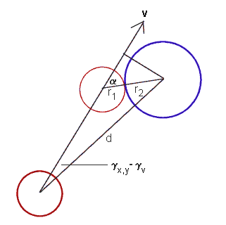
Geometry of 2D collision
If the coordinates of the balls (with radius r1 and r2) are x1,y1 and x2,y2, α is given by
(14) α = arcsin [ d.sin(γx,y-γv) / (r1+r2) ] ,
where
(15) d = √ [ (x2-x1)2 +(y2-y1)2 ] ,
(16) γx,y= arctan [ (y2-y1)/((x2-x1) ] ,
Note again that a valid solution requires |d.sin(γx,y-γv)| ≤ (r1+r2) (otherwise the balls would not collide).
The new coordinates (the position of the center of the balls at the moment of collision) are therefore
(18) x1' = x1 + vx,1.t
(19) y1' = y1 + vy,1.t
(20) x2' = x2 + vx,2.t
(21) y2' = y2 + vy,2.t
Generalization to Inelastic Collisions
(22) vx,cm = ( m1.vx,1 + m2.vx,2 )/( m1+ m2)
(23) vy,cm = ( m1.vy,1 + m2.vy,2 )/( m1+ m2)
(24) vx,1'' = (vx,1'-vx,cm).R + vx,cm
(25) vy,1'' = (vy,1'-vy,cm).R + vy,cm
(26) vx,2'' = (vx,2'-vx,cm).R + vx,cm
(27) vy,2'' = (vy,2'-vy,cm).R + vy,cm
I have tested the formulae for several cases with a Fortran Program (for those who can't use Fortran, I have also translated this into a C/C++ Version). Additionally, I have included there now also a simplified version which does not do the 'remote' collision detection illustrated above but just returns the new velocities assuming that the input coordinates are already those of the collision.
The elastic and inelastic collision in 3 dimensions can be derived in a similar way, with the only difference that now two 'impact angles' need to be defined to determine all the velocity components.